How to be the best Economic Data Scientist: The Seven Tools of Causal Inference and Ethics

Originally published on November 21, 2019, on LinkedIn, updated lightly October 29, 2022

My blog tagline is economists put the science into data science. Part of the reason I make this claim is many applied econometricians (sadly not all) place a high value on causality and causal inference. Further, those same economists will follow an ethic of working with data that is close to the 2002 guidance of Peter Kennedy and myself.

Judea Pearl discusses “The Seven Tools of Causal Inference with Reflections on Machine Learning” (cacm.acm.org/magazines/2019/3/234929), a Contributed Article in the March 2019 CACM.

This is a great article with three messages.

The first message is to point out the ladder of causation.

  1. As shown in the figure, the lowest rung is an association, a correlation. He writes it as given X, what then is my probability of seeing Y?
  2. The second rung is intervention. If I do X, will Y appear?
  3. The third is counterfactual in that if X did not occur, would Y not occur?

In his second message, he discusses an inference engine, of which he says AI people and I think economists should be very familiar. After all, economists are all about causation, being able to explain why something occurs, but admittedly not always at the best intellectual level. Nevertheless, the need to seek casualty is definitely in the economist’s DNA. I always say the question “Why?” is an occupational hazard or obsession for economists.

People who know me understand that I am a huge admirer, indeed a disciple of the late Peter Kennedy (Guide to Econometrics, chapter on Applied Econometrics, 2008). Kennedy in 2002 set out the 10 rules of applied econometrics in his article “Sinning in the Basement: What are the rules.” I think they imply practices of ethical data use and are of wider application than with Kennedy’s intended audience. I wrote about Ethical Rules in Applied Econometrics and Data Science here.

Kennedy’s first rule is to use economic theory and common sense when articulating a problem and reasoning a solution. Pearl in his Book of Why explains that one cannot advance beyond rung one without other outside information. I think Kennedy would wholeheartedly agree. I want to acknowledge Marc Bellemare for his insightful conversation on the combination of Kennedy and Pearl in the same discussion of rules in applied econometrics. Perhaps I will write about that later.

Pearl’s third message is to give his seven (7) rules or tools for Causal Inference. They are

  1. Encoding causal assumptions: Transparency and testability.
  2. Do-calculus and the control of confounding.
  3. The algorithmization of counterfactuals. 
  4. Mediation analysis and the assessment of direct and indirect effects.
  5. Adaptability, external validity, and sample selection bias.
  6. Recovering from missing data. 
  7.  Causal discovery.

I highly recommend this article, followed by the Book of Why (lead coauthor) and Causal Inference in Statistics: A Primer. (lead coauthor). Finally, I include a plug for a book in which I contributed a chapter on ethics in econometrics, Bill Franks, 97 Things About Ethics Everyone in Data Science Should Know: Collective Wisdom from the Experts.

Economic Freedom: Solve Problems, Tell Stories

Time and time again we hear employers wanting two qualities out of their data scientists, be able to solve problems and tell stories. How important is economic freedom? Does it lead to greater standards of living? The answer can be shown in tables of results well laid out, but visualizing those results has an even greater impact and better tells the story.

If a “picture is worth a thousand words” then a SAS SGPLOT is worth many pages of tables or results. Can you see the story here?

Economic Freedom is shown to be associated with ever higher standards of living across countries.

The problem is whether countries with higher levels of economic freedom also have higher standards of living. It appears that is true. The association seems undeniable. Is it causal? That is another question that the visual begs. Chicken and Egg reasoning doesn’t seem likely here. It does appeal that the association is one way. For that to be established, we have to answer is economic freedom necessary for higher standards of living. And we have to determine that if the economic freedom had not been accomplished would the standard of living not been as high.

More on that in a future post on the importance of “why.” For now, enjoy the fact that their seems to be a key to make the world better off. Oh, not just from this graph, but from countless successes in countries in the past. My undergraduate analytic students are expanding on this finding to see if their choices from the 1600 World Development Indicators of the World Bank hold up in the same way as GDP per-capita does here in this graph. We/they modify the question to “Do countries that have higher economic freedom also have greater human progress?” I am anxious to see what they find.

The Economic Freedom data comes to us from The Heritage Foundation. Let me know what you think about the visual.

This is a followup to my post on my blog at econdatascience.com “Bubble Chart in SAS SGPLOT like Hans Rosing.”

The SAS PROC SGPLOT code to create the graph is on my GITHUB repository. It makes use of Block command for the banding and selective labeling based on large residuals from a quadratic regression. The quadratic parametric regression and the loess non-parametric regression are to suggest the trend relationship.

Sorry Data not included.

Bubble Chart in SAS SGPLOT like Hans Rosing

Robert Allison blogs as the SAS Graph Guy. He recreates using SAS PROC SGPLOT the famous bubble chart from Hans Rosing of Gapminder Institute. Hans shows that life expectancy and income per person have dramatically changed over the years. Because Hans Rosing is a ot the father of visualizations, Robert produces this graph (shown here) and this very cool animation.

I can’t wait to see  Economic Freedom and income per person soon in one of these graphs. My students are trying to do this right now.  At this point in the term they are acquiring two datasets from Heritage on 168 countries, which contain the index of economic freedom for 2013 and 2018. Then they are cleaning and joining them so they can reproduce the following figure and table in SAS PROC SGPLOT for each year.


I have written about this project in prior terms here. Once they have this data joined and the above figures reproduced then they will move on to the final project for this semester. They will be looking through the 1600 World Development Indicators of the World Bank.  Each team of students will choose 5 and will join that to their data to answer the question:

Does Economic Freedom lead to greater Human Progress?

I may share their results, for now this is some pretty cool graphics from the SAS Graph Guy. 


Time Series data will lie to you, or take a random walk in Chicago.

Do you know that data lies? Come talk to me at MWSUG (Midwest SAS Users Group Conference) and I will help you protect yourself against lying data.

One of the papers i am presenting is on time series data. Time series analysis is pretty intense and there is as much art as science in its modeling. My paper is BL-101 “Exploring and characterizing time series data in a non-regression based approach.

Nobel Prize economist Ronald Coase famously said:  “If you torture the data long enough, it will confess.”  It will confess to anything, just to stop the beating. I think there is a corollary to that, “If you don’t do some interrogation, the data may just tell a lie, perhaps what you want to hear.

Consider the following graph, assembled with no torture at all and not even a short painless interrogation. The graph shows that money supply and the federal debt track each others time path very closely. It tempts you to believe what you see.  Do you believe that when the money supply increases we all have more to spend and this will translate into dept? Do you have an alternate reasoning that explains this movement? If so, this graph confirms your thoughts and you decide to use it to make or demonstrate or prove your point. Good stuff huh?

Sadly you just fell to confirmation bias and because you have failed to investigate the data generating process of the series, you fell for the lying data. You have found correlation, but not causation. in fact, you may have found a random walk.  Don’t cheer yet, that is not a good thing to make your case. 

But,” you think, “I like that graph and besides the correlation between Money Supply and Debt is really high so it has to mean something! right?

Sadly, no. 

Mathematically, if the series are random walks then changes in the series are only generated by random error. Which means the correlation between the two variables will be very low. 

A random walk takes the form of

y(t) = y(t-1) + e

which says that the currently observed variable at time t, is equal to the immediate past value plus a random error term. The problem here can be seen by subtracting y(t-1) from each side yielding a new and horrifying equation that says that any growth observed is purely random error, that is

Change in y = y(t) – y(t-1) = e.

Since you cannot write an equation to predict random error, it stands to reason that you cannot predict current or forecast future changes in the variable of interest.

Consider the next graph. The percentage change over the last year in the money supply is graphed against the percentage change over the last year of debt.  See a definite pattern? I do not. 

The correlation between money supply and debt in the first graph is 0.99 where 1.0 would be perfectly one-to-one related. In the second graph the correlation falls to 0.07 meaning there is almost no relationship between them.

The lesson: You should do more investigation, torture is not necessary, but no investigation is never desirable. 

Economists are obsessed in determining the data generating process (DGP)which take a lot of investigation. Economists know traps like random walks and know ways to find the true relationship between money supply and debt, if any. Ignore the DGP and your quick results could be a lie. Torture the data, and again you could find a lie (it just may take a long time of wasteful actions). 

So come take a random walk in Chicago with me at MWSUG. 

After the conference my paper will be available on the conference proceedings. 

A Data Science Book Adoption: Getting Started with Data Science

In my undergraduate business and economic analytics course, I have adopted Murtaza Haider‘s excellent text Getting Started with Data Science. I chose it for a lot of reasons. He is an applied econometrician so he relates to the students and me more than many authors. I truly have a very positive first impression. 

Updated: November 7, 2020

On my campus you can hear economics is not part of data science, they don’t do data science, that is, data science belongs to the department of statistics (no to the engineers, to the computer science department, and on and on like that.)  We have come a long way, but years ago, for example, the university launched a major STEM initiative and the organizers kept the economic department out of it even though we ask to be part of it. Of course, when they did their big role out, without our department, they brought in a famous keynote speaker who was … wait for it … an economist.

My department , just launched a Business Data Analytic economics degree in the College of Business Administration at the University of Akron.  We see tech companies filling up their data science teams with economists, many with PhDs. Our department’s placements have been very robust in the analytic world of work. My concern is seeing undergraduates in economics get a start in this field. and Murtaza Haider offers a nice path. 

Dr. Haider, has a Ph.D. in civil engineering, but his record is in economics, specifically in regional and urban, transportation and real-estate, and he is a columnist for the Financial Post. and I can attest to his applied econometrics knowledge based on his fine book which I explore below.

WHAT IS DATA SCIENCE

Haider has a broad idea of what is data science and follows a well-reasoned path on how to do data science. Like my approach to this class, he is heavy into visualizations through tables and graphics and while I would appreciate more design, he makes an effort to teach the communicative power of those visualizations. Also, like me, he is highly skeptical of the value of learning to appease the academic community at the expense of serving the business (non-academic) community where the jobs are. I really appreciate that part of it.

PROBLEM SOLVING AND STORYTELLING

He starts with storytelling. our department recognizes that what our economists do, what they do to bring value is they know how to solve problems and tell stories. Again this is a great first fit. He then moves to Data in a 24/7 connected world. He spends considerable time on data cleaning and data manipulation. Again I like how he wants students to use real data with all of its uncleanliness to solve problems. Chapter 3 focuses on the deliverables part of the job and again I think he is spot on. 

Then through the remaining chapters he first builds up tables, then graphs, and onto advanced tools and techniques. My course will stop somewhere in the neighborhood of chapter 8.

(Update: Chapter 8 begins with the binary and limited dependent variables, and full disclosure my last course did not begin this chapter, we ended in Chapter 7 on Regression). Perhaps the professor in the next course will consider Getting Started in Data Science for Applied Econometrics II.  (Update: Our breakdown in our Business Data Analytics economics degree is that Econometrics I is heavily coding and application-based, while econometrics II is a more mathematical/ theoretical based course with intensive data applications.  It is a walk before you run approach, building up an understanding of analysis and data manipulation first. )

I use a lot of team-based problem-based learning in my instruction and Haider’s guidance through the text is instructing teams how to think through problems to get one of many possible solutions, not highlighting only one solution. In this way, he reinforces both creativity in problem-solving. I like what I read, I wonder what I will think after students and I go through it this term. (Update: I/we liked the text, but did not follow it page by page.  The time constraint of the large data problem began to dominate and crowd out other things, hence why I did not get to Chapter 8, my proposed end. However, because in course 1 which emphasizes data results over theoretical knowledge, I was well pleased.)

PROBLEM ARTICULATION, DATA CLEANING, AND MODEL SPECIFICATION

Another reason I like the book so much is he cites Peter Kennedy, the now passed, research editor for the Journal of Economic Education. Peter was very influential on me and applied econometricians who really want to dig into the data. Most of my course is built around his work and especially around the three pillars of Applied Econometrics.: (1) the ability to articulate a problem, (2) the need to clean data, and (3) to focus deeply on model specification. He argues that most Ph.D. programs fail to teach the applied, allowing their time to focus on theoretical statistics and propertied of inferential statistics. Empirical work is often extra and conducted, even learned, outside of class. I have never taught like that (OK, maybe my first year out of my Ph.D.), but my last 40 years have been a constant striving to make sure my students are prepared for the real as opposed to the academic world. Peter made all the difference bringing my ideas into sharp focus. I like Haider’s work, Getting Started with Data Science, because it is written like someone who also holds the principles put forth by Peter Kennedy in high regard. 

SOFTWARE AGNOSTIC, BUT TOO MUCH STATA AND NOT ENOUGH SAS

On page 12 he gets much credit for saying he does not choose only one software, but includes “R, SPSS, Stata and SAS.” I get the inclusion of SPSS given it is IBM Press, but there is virtually no market for Stata (or SPSS)  in the state of Ohio or 100 miles around my university’s town of Akron, OH. Also, absent is python, which is in heavy use in the job market.  You can see the number of job listings mentioning each program in the chart below. 

I am highly impressed with Haider’s book for my course, but that does not extend to everything in the book. My biggest peeve is his heavy use of Stata. I would prefer a text that highlights the class language (SAS) more and was more sensitive to the market my students will enter.  

Stata is a language adopted by nearly all professional economists in the academic space and in the journal publication space, however, I think this use is misguided when the book is to be jobs facing and not academic facing. While he shows plenty of R, there is no python and no SAS examples. All data sets are available on his useful website, but since SAS can read STATA data sets that isn’t much of a problem.

Numbers for all of indeed.com listings in August 2019: Python, 70K; R 52K; SAS 26K, SPSS 3,789; Stata 1,868

SAS Academic Specialization

Full disclosure, we are a SAS school as part of the SAS Global Academic Program and offer both a joint SAS certificate to our students as well as offering them a path to full certification. 

(Update: The SAS joint certificate program has been rebranded and upgraded to the SAS Academic Specialization and is still a joint partnership between the college or university and SAS, but now in three tiers of responsibilities and benefits. We are at tier 3 and the highest level. Hit the link for more details.) 

We also teach R as well in our forecasting course and students are exposed to multiple other programs over their career including SQL, Tableau, Excel (for small data handling, optimization, and charting/graphics), and more. 

Buy This Book

Most typical econometric textbooks are in the multiple hundreds of dollars (not kidding) and almost none are suitable to really prepare for a job in data science. This book on Amazon is under $30 and is a great practical guide. Is it everything one needs? Of course not, but at the savings from $30 you can afford many more resources.

More SAS Examples

So it is natural given our thrust as a SAS School, that I would have preferred examples in SAS to assist the students. Nevertheless, I accepted the challenge to have students develop the SAS code to replicate examples in the book. This is a great way to avoid too much grading of assignments. Let them read Haider’s examples, say a problem that he states, and then solves with STATA. He presents both question and answer in STATA and my student’s task is to answer the problem in SAS. They can self check and rework until they come to the right numerical answer, and I am left helping only the truly lost.  

Overall, I love the outline of the book. I think it fits with a student’s first exposure to data science and I will know more at the end of this term. I expect to be pleased. (Update: I was.) 

If you are at all in data science and especially if you have a narrow idea that data science is only Machine Learning or big data, you need to spend time with this book, specifically read the first three chapters and I think you will have your eyes opened and a better appreciation of the field of data science.

Testing for a structural break

Ever throw a dummy variable in a regression to see whether the effect the dummy variable is measuring has an impact on the dependent variable? Ever find that the dummy variable had the wrong sign, was of small magnitude or had vastly large variance so that you decided based on your data that the effect measured by the dummy variable had no effect? Of course you have, we all have.

But did you know that your data may be lying to you?

This presentation is an exploration of whether a time series changes based on an intervention that occurs half way through the data. Perhaps the intervention is a new law, or a treatment of some kind, did it have an effect. In our example, the dummy variable is insignificant in the first instance, model specification is in doubt and a full-on testing strategy is developed. That is, the test of whether D, the dummy variable, effects Y, the outcome measure is more than a p-test in a simple single regression, much more. Check out the classroom presentation and I will eventually load all the SAS code here to run all 8 regressions required and the multiple tests of each regression to answer the original hypothesis that D matters.

Susan Athey on the Impact of Machine Learning on Econometrics and Economics (part 2)

I posted Susan Athey’s 2019 Luncheon address to the AEA and AFA in part 1 of this post.  (See here for her address).

Now, in part 2, I post details on the continuing education Course on Machine Learning and Econometrics from 2018 featuring the joint efforts of Susan Athey and Guido Imbens.

It relates to the basis for this blog where I advocate for economists in Data Science roles. As a crude overview, ML uses many of the techniques known by all econometricians and has grown out of data mining and exploratory data analysis, long avoided by economists precisely because such methods lead to in the words of Jan Kmenta “beating the data until it confesses.” ML also makes use of AI type methods that started with brute force methods noting that the computer can be set lose on a data set and in a brutish way try all possible models and predictions seeking a best statistical fit, but not necessarily the best economic fit since the methods ignore both causality and the ability to interpret the results with a good explanation.  

Economists historically have focused on models that are causal and provide the ability to focus on the explanation, the the ability to say why. Their model techniques are designed to test economic hypotheses about the problem and not just to get a good fit. 

To say we have discussed historically the opposite ends of a fair coin by setting up the effect of X–>y is not too far off. ML focuses on y and econometrics focus on X. The future is focusing on both, the need to focus good algos on what is y and the critical understanding of “why” which is the understanding of the importance of X.  

This course offered by the American Economic Association just about one year ago, represents the state of the art of the merger of ML and econometrics.  I offer it here (although you can go directly to the AEA website) so more can explore how economists need to incorporate the lessons of ML and of econometrics and help produce even stronger data science professionals. 

AEA Continuing Education Short Course: Machine Learning and Econometrics, Jan 2018

Course Presenters

Susan Athey is the Economics of Technology Professor at Stanford Graduate School of Business. She received her bachelor’s degree from Duke University and her PhD from Stanford. She previously taught at the economics departments at MIT, Stanford and Harvard. Her current research focuses on the  intersection of econometrics and machine learning.  As one of the first “tech economists,” she served as consulting chief economist for Microsoft Corporation for six years.

Guido Imbens is Professor of Economics at the Stanford Graduate School of Business. After graduating from Brown University Guido taught at Harvard University, UCLA, and UC Berkeley. He joined the GSB in 2012. Imbens specializes in econometrics, and in particular methods for drawing causal inferences. Guido Imbens is a fellow of the Econometric Society and the American Academy of Arts and Sciences. Guido Imbens has taught in the continuing education program previously in 2009 and 2012.

Two day course in nine parts - Machine Learning and Econometrics, Jan 2018

 Materials:

Course Materials (will attach to your Google Drive)

The syllabus is included in the course materials and carries links to 4 pages of readings which are copied and linked to the source articles below.

Webcasts:

View Part 1 – Sunday 4.00-6.00pm: Introduction to Machine Learning Concepts 

(a) S. Athey (2018, January) “The Impact of Machine Learning on Economics,” Sections 1-2. 

(b) H. R. Varian (2014) “Big data: New tricks for econometrics.” The Journal of Economic Perspectives, 28 (2):3-27.

(c) S. Mullainathan and J. Spiess (2017) “Machine learning: an applied econometric approach” Journal of Economic Perspectives, 31(2):87-106  

View Part 2 – Monday 8.15-9.45am: Prediction Policy Problems

(a) S. Athey (2018, January) “The Impact of Machine Learning on Economics,” Section   3. 

(b) S. Mullainathan and J. Spiess (2017) “Machine learning: an applied econometric approach.” Journal of Economic Perspectives, 31(2):87-106. 


View Part 3 – Monday 10.00-11.45am: Causal Inference: Average Treatment Effects

(a) S. Athey (2018, January) “The Impact of Machine Learning on Economics,” Section 4.0, 4.1. 

(b) A. Belloni, V. Chernozhukov, and C. Hansen (2014) “High-dimensional methods and inference on structural and treatment effects.” The Journal of Economic Perspectives, 28(2):29-50. 

(c) V. Chernozhukov, D. Chetverikov, M. Demirer, E. Duo, C. Hansen, W. Newey, and J. Robins (2017, December) “Double/Debiased Machine Learning for Treatment and Causal Parameters.” 

(d) S. Athey, G. Imbens, and S.Wager (2016) “Estimating Average Treatment Effects: Supplementary Analyses and Remaining Challenges.”  Forthcoming, Journal of the Royal Statistical Society-Series B.

View Part 4 – Monday 12.45-2.15pm: Causal Inference: Heterogeneous Treatment Effects

(a) S. Athey (2018, January) “The Impact of Machine Learning on Economics,” Section 4.2. 

(b) S. Athey, G. Imbens (2016) “Recursive partitioning for heterogeneous causal effects.” Proceedings of the National Academy of Sciences, 113(27), 7353-7360.

View Part 5 – Monday 2.30-4.00pm: Causal Inference: Heterogeneous Treatment E ects, Supplementary Analysis

(a) S. Athey (2018, January) “The Impact of Machine Learning on Economics,” Section 4.2, 4.4. 

(b) S. Athey, and G. Imbens (2017) “The State of Applied Econometrics: Causality and Policy Evaluation,” Journal of Economic Perspectives, vol 31(2):3-32.

(c) S. Wager and S. Athey (2017) “Estimation and inference of heterogeneous treatment effects using random forests.” Journal of the American Statistical Association 

(d) S. Athey, Tibshirani, J., and S.Wager (2017, July) “Generalized Random Forests

(e) S. Athey, and Imbens, G. (2015) “A measure of robustness to misspeci cation.” The American Economic Review, 105(5), 476-480.

View Part 6 – Monday 4.15-5.15pm: Causal Inference: Optimal Policies and Bandits

(a) S. Athey. (2018, January) “The Impact of Machine Learning on Economics,”
Section 4.3. 

(b) S. Athey and S. Wager (2017) “Efficient Policy Learning.”

(c) M. Dudik, D. Erhan, J. Langford, and L. Li, (2014) “Doubly Robust Policy
Evaluation and Optimization” Statistical Science, Vol 29(4):485-511.

(d) S. Scott (2010), “A modern Bayesian look at the multi-armed bandit,” Applied Stochastic Models in Business and Industry, vol 26(6):639-658.

(e) M. Dimakopoulou, S. Athey, and G. Imbens (2017). “Estimation Considerations in Contextual Bandits.” 

View Part 7 – Tuesday 8.00-9.15am: Deep Learning Methods

(a) Y. LeCun, Y. Bengio and G. Hinton, (2015) “Deep learning” Nature, Vol. 521(7553): 436-444.

(b) I. Goodfellow, Y. Bengio, and A. Courville (2016) “Deep Learning.” MIT Press.

(c) J. Hartford, G. Lewis, K. Leyton-Brown, and M. Taddy (2016) Counterfactual
Prediction with Deep Instrumental Variables Networks.” 

View Part 8 – Tuesday 9.30-10.45am: Classi cation

(a) L. Breiman, J. Friedman, C. J. Stone R. A. Olshen (1984) “Classi cation and
regression trees,” CRC press.

(b) I. Goodfellow, Y. Bengio, and A. Courville (2016) \Deep Learning.” MIT Press.

View Part 9 – Tuesday 11.00am-12.00pm: Matrix Completion Methods for Causal Panel Data Models

(a) S. Athey, M. Bayati, N. Doudchenko, G. Imbens, and K. Khosravi (2017) “Matrix Completion Methods for Causal Panel Data Models.” 

(b) J. Bai (2009), “Panel data models with interactive fi xed effects.” Econometrica, 77(4): 1229{1279.

(c) E. Candes and B. Recht (2009) “Exact matrix completion via convex optimization.” Foundations of Computational Mathematics, 9(6):717-730.


Susan Athey on the Impact of Machine Learning on Econometrics and Economics (part 1)

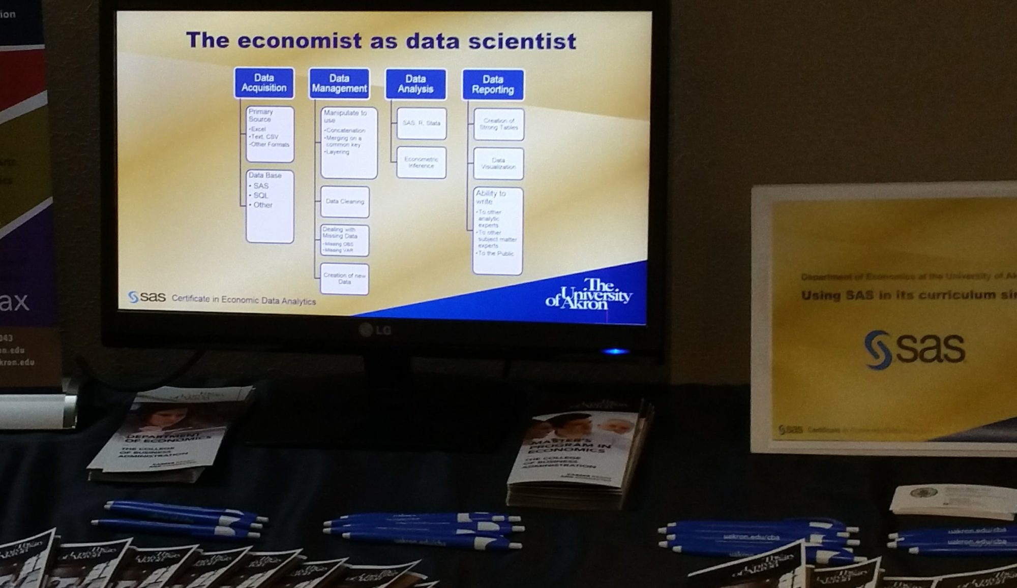
Economists make great data scientists. In part, this is because they all are trained in the four pillars of data science (1) data acquisition, (2) Data manipulation, cleaning and management, (3) analysis and (4) reporting and visualization. Good programs make sure that the economics students are trained in all four areas. Economists have subject matter expertise that is wrapped in a formalized way of thinking and problem solving ability. Quick answer, why are economists so valuable in business? – They know how to solve problems and tell stories from the evidence. 

As to the analysis part of these pillars, economists are typically wrapped in causality and explanation of X in the y = f(X,e) model. Economists in forecasting become more interested in predicting y with less or much less on the factors X

When I talk to many I hear data science being linked only with Machine Learning as if ML and data science are synonyms. This is far from the truth, with Data Science being very broad and ML a specific way and in some cases a dominate way of approaching a data problem. ML is making its way into economic curriculum. So what is the role of ML in economics now and into the future and more particularly the role between econometrics and ML?

No one in the economics profession knows more about the intersection of economics and machine learning than Susan Athey who just last month gave an address to the American Economic Association and the American Finance Association.  I am posting this address so you may understand the current state. 

In part 2 of this post I link to her two day course offered in January 2018 on ML and Econometrics with Guido Imbens. 

The AEA/AFA address, Jan 2019

This video was captured at the joint luncheon for the American Economics Association and the American Finance Association that occurred at the January 2019 Annual Meetings in Atlanta. 

Susan Athey who is The Economics of Technology Professor of the Graduate School of Business at Stanford University delivers the address and is introduced by Ben Bernanke, former FED chair, now at the Brookings Institution.

external link: https://www.aeaweb.org/webcasts/2019/aea-afa-joint-luncheon-impact-of-machine-learning

Economists as engineers: A new Chapter

(0:59:25) “The AI and econometric theory need work, but they are not the main constraint…. Instead the success is going to depend on understanding the context, understanding the setting….

“(The economist can be) motivated by social science research about where should I be spending my time, where should I be intervening? (Economists need) to use empirical work to help figure out what the best opportunities are.

Economists can help with defining measures of success.  We need to recognize that AI has billions of ways to optimize so we better be telling the algo the right thing. Those algos need to be constrained and informed by 

(1:01:22)  “Broadly, when economists return to their institutions that are building AI and data science initiatives that … the social scientists (she thinks)  are going to be more important than the  computer scientist in terms of what is the conceptual thing, what is the thing that makes something succeed or fail, that makes it screw up and have adverse consequences versus being really successful and impactful. We (economists) are going to need to join interdisciplinary teams and the evaluation will be embedded and not separable from the system. So that means we are going to have the opportunity to intervene in the world like we never have before. But it also comes great responsibility because we will be the people in the room who really can understand the good and the bad and make sure it happens in a safe way.””


David Autor on Changing Patterns of Work

Are earnings differences between males and females due to discrimination? A typical approach is to compare the earnings of women to that of men and try to control for typical understandable differences such as education level and location and other factors. Perhaps education levels and location interact and an interaction term is introduced into our model. However, the largest assumption is that once we define our variables, homogeneity rules, that education is homogeneous, e.g., HS graduation means the same for all groups, over all times and locations). I see Autor’s lecture pointing out this heterogeneity and disputing the assumption that all persons are products of the same data generating process. He takes this on and at least for me smashes my initial biases. To be fair, this is my reading of his efforts, he does not utter the word heterogeneity at all, but I don’t think he needed to, not everyone in the audience are econometricians and the implicit heterogeneity problem is taken on directly. I will be sharing this lecture with my data analytic students as a great example of exploratory data analysis that allows a masterfully told story through complex preparation and easy to understand visuals.

The Richard T. Ely lecture at the 2019 American Economic Association meetings was presented by David H. Autor (MIT, NBER) comparing Work of the Past with the Work of the Future. Motivated in part by the “remarkable rise of wage inequality by education,” “vast increase in supply of educated workers,” and a “key observation (of the) polarization of work” that while “most occupational reallocation is upward,” “the occupational mobility is almost exclusively downward” for non-college workers, Autor proceeds to give rise to answers to the questions surrounding

  1. Diverging earnings and diverging job tasks
  2. The changing geography of work and wages
  3. The changing geography of workers, and
  4. What and where is the work of the future.

The visual presentation makes his data exploration very understandable and are masterfully done. He truly paints a picture that emerges from a vast amount of data that is entertaining and informative. This is well worth the 47 minutes and may actually challenge your preconceived thinking as to the nature of inequality in earnings. It is not as simple as one may think and he perfectly illustrates without ever uttering the word that data heterogeneity when ignored leads to false and inescapable conclusions.

Work of the past, work of the future. Richard T. Ely Lecture, AEA meetings, Atlanta, January 4, 2019.

Click on the above image and you will be well rewarded if you want to see a story told with strong graphics, proving to me anyway, that deep diving into data and presenting simple graphics (although complex in their creation) is a most effective way to communicate. A couple of examples of the graphics:

What if we do an econometric analysis of earnings between men and women using current data and a similar analysis from the 1980s. Can you see how this graph as one of many in Autor’s presentation might create havoc in comparing the result in the 1980s to one current? Watch the presentation, plenty of more visuals like this one.